Principal Component Analysis

1st January, 2025•Machine Learning

---

The Curse of Dimensionality

The curse of dimensionality refers to various phenomena that arise when working with data in high-dimensional spaces that do not occur in low-dimensional settings, such as three-dimensional physical space.

• In high-dimensional space, data points are increasingly sparse, meaning that most training instances are likely to be far away from each other.
• This sparsity makes predictions less reliable as they are based on larger extrapolations.
• The increased sparsity and distance between data points also leads to a greater risk of overfitting the data.

A theoretical solution to the curse of dimensionality would be to increase the size of the training set to achieve a sufficient density of data points. However, this is impractical as the number of training instances required to reach a given density grows exponentially with the number of dimensions.

How the Curse of Dimensionality Affects Machine Learning Systems

The curse of dimensionality can make it difficult for machine learning algorithms to find patterns in the data because the data points are so spread out.

This can lead to longer training times and reduced accuracy.

It can also lead to overfitting, where the model learns the training data too well and does not generalize well to new data.

This is because in high-dimensional spaces, there are many more ways for a model to fit the data, even if the data is random noise.

Dimensionality Reduction

One approach to addressing the curse of dimensionality is dimensionality reduction. Dimensionality reduction algorithms attempt to reduce the number of features in a dataset while preserving as much information as possible. Two main approaches are: one for linear data and non-linear data. We would only be focusing on linear data for today, specically, Principal Component Analysis

Principal Component Analysis (PCA)

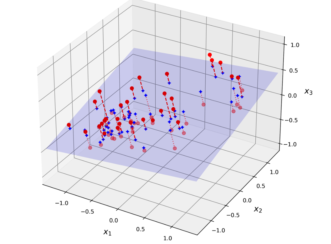
PCA seeks to identify a lower-dimensional subspace that captures the maximum variance in the original high-dimensional data. 5Image reference from Hands On Machine Learning Book by Aurélien Géron(Image reference from Hands On Machine Learning Book by Aurélien Géron)

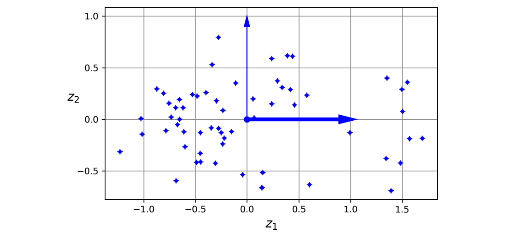
This is done by finding the eigenvectors of the data covariance matrix. The eigenvectors corresponding to the largest eigenvalues capture the dimensions of greatest variance, and these eigenvectors form the principal components.

Projecting the data onto the principal components results in a lower-dimensional representation of the data that retains as much variance as possible. 6Image reference from Hands On Machine Learning Book by Aurélien Géron(Image reference from Hands On Machine Learning Book by Aurélien Géron)

Mathematical Formulation

Given a data matrix $X$ with $N$ data points, each with $D$ features, PCA proceeds as follows:

1. Center the data:

Calculate the mean of the data, $\mu = \frac{1}{N}\sum_{n=1}^{N}x_n$, and subtract it from each data point: $x_n \leftarrow x_n - \mu$.

2. Compute the covariance matrix:

The covariance matrix $\Sigma$ is a $D \times D$ matrix that measures the pairwise covariances between the features. It is calculated as follows:

$\Sigma = \frac{1}{N}X^TX$

3. Perform eigen-decomposition:

Find the eigenvalues ($\lambda_i$) and eigenvectors ($v_i$) of the covariance matrix. The eigenvectors form an orthonormal basis, meaning they are orthogonal to each other and have unit length. The eigenvalues represent the amount of variance explained by each eigenvector.

4. Select principal components:

Choose the $L$ eigenvectors corresponding to the $L$ largest eigenvalues, where $L$ is the desired dimensionality of the reduced data. These eigenvectors form the matrix $W_L$.

5. Project the data:

Project the data onto the principal components to obtain the reduced data matrix $Z$: $Z = XW_L$

The columns of $Z$ are the coordinates of the data points in the lower-dimensional subspace defined by the principal components.

Explained Variance Ratio

The explained variance ratio for each principal component indicates the proportion of variance in the dataset captured by that component. It can be calculated as:

$\text{EVR}_i = \frac{\lambda_i}{\sum_{j=1}^{D}\lambda_j}$

The explained variance ratio of a principal component (PC) indicates the proportion of the dataset's variance that lies along the principal component. The explained variance ratio is available in the explained_variance_ratio_ variable after fitting the PCA transformer to the dataset.

For instance:

• A 3D dataset is projected onto the 2D plane defined by the first two principal components.
• After fitting the PCA transformer, the explained variance ratios for the first two components are 0.76 and 0.15, respectively.
• This output means that 76% of the dataset's variance lies along the first PC, and 15% lies along the second PC.

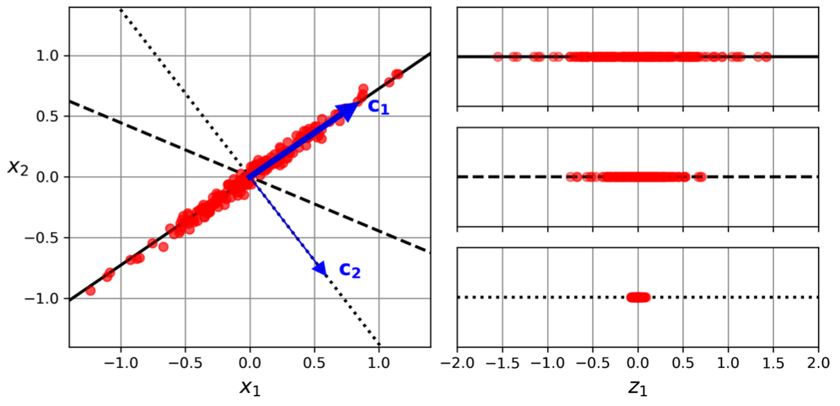
This leaves about 9% for the third PC. This information can be used to decide whether to drop the third PC as it carries little information.7It seems reasonable to select the axis that preserves the maximum amount of variance.(It seems reasonable to select the axis that preserves the maximum amount of variance.)

Choosing the Number of Dimensions

The number of principal components, $L$, determines the dimensionality of the reduced data. This can be chosen by setting a threshold for the cumulative explained variance ratio (e.g., 95%) or by examining a plot of the explained variance as a function of the number of dimensions and identifying an elbow where the explained variance stops growing rapidly.

Reconstruction

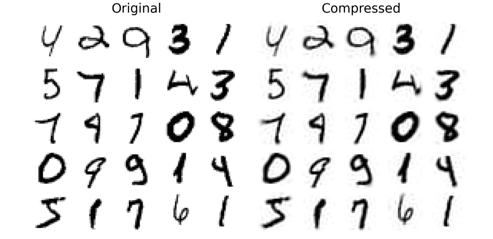
After dimensionality reduction, the training set takes up much less space. For example, applying PCA to the MNIST dataset while preserving 95% of its variance results in 154 features instead of the original 784. This means the dataset is now less than 20% of its original size, and only 5% of variance was lost!

It is also possible to decompress the reduced dataset back to 784 dimensions by applying the inverse transformation of the PCA projection. This will not give you back the original data, since the projection lost a bit of information (within the 5% variance that was dropped), but it will likely be close to the original data. 8Image reference from Hands On Machine Learning Book by Aurélien Géron(Image reference from Hands On Machine Learning Book by Aurélien Géron)

The mean squared distance between the original data and the reconstructed data (compressed and then decompressed) is called the reconstruction error.

The original data can be approximately reconstructed from the reduced data by applying the inverse transformation, which involves multiplying the reduced dataset $X_{d-proj}$ by the transpose of the matrix $W_d$:

$X_{\text{recovered}} = X_{d-proj}W_d^T$

Relevance of PCA

PCA is a powerful technique with several key applications:

1. Dimensionality Reduction: Reduces the number of features while retaining as much variance as possible, making data more manageable.
2. Noise Reduction: Filters out noise by focusing on the principal components that capture the most variance.
3. Multicollinearity Handling: Transforms correlated features into uncorrelated components, useful for algorithms like linear regression.
4. Visualization: Projects high-dimensional data into 2D or 3D space for easier visualization and pattern recognition.
5. Feature Extraction: Creates new features (principal components) that are linear combinations of the original features.
6. Efficiency: Speeds up machine learning algorithms and reduces memory usage by reducing dimensionality.

Where PCA is Most Useful

PCA is particularly useful in the following scenarios:

1. Exploratory Data Analysis (EDA): Identifies patterns and relationships in high-dimensional data.
2. Image Processing: Used for tasks like face recognition (eigenfaces) and image compression.
3. Genomics and Bioinformatics: Analyzes gene expression data to identify key genes or patterns.
4. Finance: Identifies principal components of asset returns for portfolio optimization.
5. Natural Language Processing (NLP): Reduces dimensionality of word embeddings or document-term matrices.
6. Signal Processing: Separates signals from noise in applications like speech recognition and EEG analysis.
7. Anomaly Detection: Helps identify outliers or anomalies in the data.
8. Preprocessing for Machine Learning: Improves performance and efficiency of algorithms like k-means, SVMs, and neural networks.

Limitations of PCA

1. Linear Assumption: PCA assumes that the data lies on a linear subspace. For nonlinear relationships, techniques like Kernel PCA or t-SNE may be more appropriate.
2. Interpretability: Principal components are linear combinations of the original features, which can make them difficult to interpret.
3. Variance vs. Importance: Directions of maximum variance may not align with the most important features for a specific task (e.g., classification).
4. Sensitive to Scaling: PCA is sensitive to the scale of the features, so data should be standardized before applying PCA.

Practical Tips for Using PCA

1. Standardize the Data: Always standardize the data (mean = 0, variance = 1) before applying PCA, especially when features are on different scales.
2. Choose the Right Number of Components: Use the explained variance ratio or a scree plot to determine the optimal number of principal components.
3. Visualize the Results: Plot the first two or three principal components to visualize the data and identify clusters or patterns.
4. Combine with Other Techniques: Use PCA in combination with other techniques (e.g., clustering, classification) to enhance their performance.