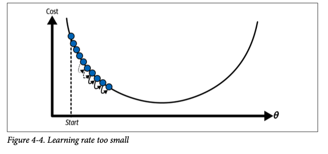
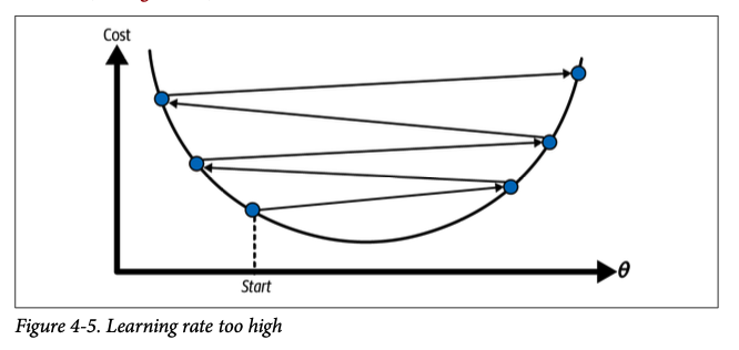
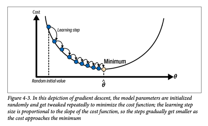
Gradient Descent

16th November, 2024•Machine Learning

GD is a more general optimization algorithm that gradually tweaks the model parameters to minimize the cost function. Stochastic Gradient Descent (SGD) is particularly efficient for large datasets as it updates parameters based on a single instance or a small batch of instances at a time.

The Basic Idea of Gradient Descent

Imagine trying to find the lowest point in a valley while you're blindfolded. You can only feel the slope of the ground beneath your feet. A reasonable strategy would be to take small steps in the direction where the ground slopes downward. This is essentially what gradient descent does. It aims to find the values for the model parameters that minimize a cost function (a function that measures how much error the model is making).

Here's how it works in the context of linear regression, which is the focus of the video:

1. Start with a guess: Begin with an initial guess for the model's parameters (θ). These are often randomly initialized.
1. Calculate the gradient: The gradient of the cost function tells you the direction of the steepest ascent. In other words, it indicates how you should change the parameters to increase the error the most. You want to move in the opposite direction to decrease the error.
1. Update the parameters: Adjust the parameters (θ) by taking a small step in the direction opposite to the gradient. The size of this step is determined by the learning rate (η).
1. Repeat until convergence: Continue steps 2 and 3 until the parameters converge to a minimum of the cost function. This is usually when further updates result in negligible improvement in the model's performance.

Learning Rate An important parameter in gradient descent is the size of the steps, determined by the learning rate hyperparameter. If the learning rate is too small, then the algorithm will have to go through many iterations to converge, which will take a long time

Not all cost functions are simple: Instead of resembling a smooth bowl, some cost functions can have irregular landscapes with holes, ridges, and plateaus. This irregularity can lead to challenges in converging to the global minimum.

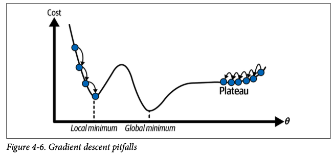
Image Alt1gradient descent algorithms can face when trying to reach the global minimum of a cost function.(gradient descent algorithms can face when trying to reach the global minimum of a cost function.)

Local Minimum Trap: A key challenge arises when the cost function has local minima. A local minimum is a point where the function is lower than its immediate surroundings but not necessarily the lowest point overall. If the algorithm starts at or near a local minimum, it might converge there and get stuck, failing to find the global minimum.

Mathematical Representation of Gradient Descent

The gradient descent update rule is given by:

\theta_{N+1} = \theta_{N} - \alpha \nabla_{\mathbf{\theta}}\operatorname{MSE}(\mathbf{\theta})

where:

$\theta_{N+1}$ represents the updated parameter vector.
$\theta$ is the current parameter vector.
$\alpha$ is the learning rate (a hyperparameter that controls the step size).
$\nabla_{\mathbf{\theta}}\operatorname{MSE}(\mathbf{\theta})$ is the gradient vector of the Mean Squared Error (MSE) cost function with respect to the parameter vector $\theta$ .

The gradient vector points in the direction of the steepest ascent of the cost function. By subtracting it from the current parameter vector, we move the parameters in the direction that decreases the cost function (downhill in our valley analogy).

Gradient Descent Implementation python

import numpy as np

np.random.seed(42)

m = 100
X = np.random.rand(m, 1)
y = 4 + 3 * X + np.random.rand(m, 1)


eta = .271828 # learning rate
n_epochs = 1000
m = len(X_b) # number of instances

theta = np.random.randn(2, 1) # our initial guess for theta

# randomly initialized model parameters
for epoch in range(n_epochs):
    gradients = 2 / m * X_b.T @ (X_b @ theta - y) # MSE value
    theta = theta - eta * gradients

Values for theta as computed would be:

array([[4.51359766],
       [2.96646836]])

2Code Snippet from Hands On Machine Learning Book by Aurélien Géron(Code Snippet from Hands On Machine Learning Book by Aurélien Géron)

Types of Gradient Descent

Batch Gradient Descent

This type calculates the gradient of the cost function using the entire training dataset at each iteration. This leads to a more stable convergence towards the global minimum, especially for convex cost functions. The Normal Equation, though not iterative like gradient descent, also uses the whole dataset to directly calculate the optimal θ. However, using the entire dataset for each step makes this method computationally expensive for large datasets.

Advantages: Can find the true minimum for convex cost functions.
Disadvantages: Slow for large datasets as it needs to process all the data in each iteration.

Stochastic Gradient Descent (SGD)

In contrast to batch gradient descent, SGD randomly selects a single instance from the training set in each iteration and computes the gradient based on that single instance. While this makes SGD much faster, especially for large datasets, the updates to the parameter values become noisy and the path toward the minimum less stable. Despite not converging as smoothly as batch gradient descent, SGD might be better at escaping local minima due to its stochastic nature.

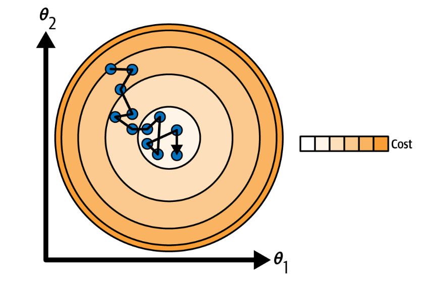
Stochastic Gradient Descent Implementation python

n_epochs = 50
t0, t1 = 5, 50

def learning_schedule(t):
    return t0 / (t + t1)

theta = np.random.randn(2, 1)

for epoch in range(n_epochs):
    for iteration in range(m):
        random_index = np.random.randint(m)
        xi = X_b[random_index : random_index + 1]

        yi = y[random_index : random_index + 1]
        gradients = 2 * xi.T @ ( xi @ theta - yi)

        eta = learning_schedule(epoch * m + iteration)
        theta = theta - eta * gradients

3Code Snippet from Hands On Machine Learning Book by Aurélien Géron(Code Snippet from Hands On Machine Learning Book by Aurélien Géron)

Advantages: Much faster than batch GD, can handle large datasets. Has a better chance of escaping local minima due to its randomness.
Disadvantages: The parameter updates are noisy, resulting in a less stable path towards the minimum. May not converge perfectly to the global minimum, but might oscillate around it.

Mini-Batch Gradient Descent

This approach combines aspects of both batch and stochastic gradient descent. Instead of using the entire dataset or a single instance, it uses a small, randomly selected batch of training instances (typically between 10 and 100) to compute the gradient at each iteration. By using a batch, mini-batch gradient descent attempts to leverage hardware optimizations for matrix operations, potentially leading to faster training than batch gradient descent. While it might not converge as precisely to the global minimum, it generally oscillates in a smaller region around it compared to SGD.

Advantages: Combines the speed of SGD with the stability of batch GD. Can benefit from hardware optimizations (especially on GPUs), making it faster than batch GD.
Disadvantages: May not find the exact minimum, but might settle in a region close to it. The choice of mini-batch size can impact performance.

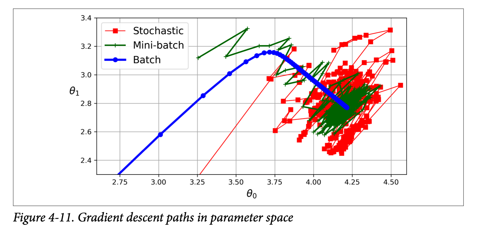
Choosing the Right Gradient Descent Algorithm

The choice of gradient descent algorithm depends on factors like the size of the dataset, the computational resources available, and the nature of the cost function.

Small datasets: Batch gradient descent is generally a good choice.
Large datasets: Mini-batch gradient descent or stochastic gradient descent offer better performance.
Highly irregular cost functions: Stochastic gradient descent might be preferred as it can better escape local minima.